Teaching a DIY Manipulator to Move with Physics: Euler–Lagrange Control on the MMV1


Introduction
The Marcinczyk Manipulator V.1. (M.M.V.1) is a four-degree-of-freedom robotic manipulator developed to investigate the relationship between rigid-body dynamics, electromechanical actuator behavior, and low-level feedback control. Its independent generalized coordinates are defined as

where r represents the radial prismatic displacement, θ1 and θ2 describe the primary revolute-joint motion, and ϕ represents the azimuthal rotation of the manipulator base. The system is modeled using an Euler–Lagrange formulation that incorporates the measured link masses, centers of mass, inertia tensors, actuator gearing, armature resistance, back-electromotive-force effects, and gravitational loading. The resulting equations are mapped directly into normalized motor duty-cycle commands, allowing the dynamical model to serve as a nominal feedforward component within the low-level controller.
The angular coordinates θ1, θ2, ϕ are measured using AS5048A magnetic rotary encoders. These sensors provide absolute angular-position measurements at the corresponding drivetrain locations, after which the encoder readings are corrected using experimentally determined zero offsets, sign conventions, and gear ratios to recover the rigid-body joint coordinates. The radial coordinate r is measured using a B10K linear potentiometer mechanically coupled to the linear-actuator stroke. Its analog output is sampled by the Teensy 4.1 and mapped to the calibrated physical displacement of the prismatic coordinate.
Joint velocities and accelerations are obtained through numerical differentiation of the measured position signals, together with filtering and magnitude limits intended to reduce amplification of encoder and analog-measurement noise. These estimated states are supplied to the Euler–Lagrange duty-cycle model and to the proportional–derivative feedback controller. The complete low-level control law combines model-based feedforward compensation with measured-state feedback, enabling the Teensy 4.1 to compute actuator commands directly from desired joint-space trajectories.
This structure separates high-level trajectory generation from low-level dynamical control. Cartesian references obtained from vision, SLAM, path planning, or external serial commands may first be converted into feasible generalized-coordinate trajectories using inverse kinematics. The corresponding desired position, velocity, and acceleration histories are then passed to the embedded inverse-dynamics controller. As a result, the external planning system does not need to reproduce the full manipulator dynamics; it needs only to provide a kinematically feasible reference, while the onboard Euler–Lagrange model supplies most of the nominal actuation required to follow that trajectory.
Mathematical Analysis
Euler-Lagrange Dynamics
The derivations for the M.M.V.1. has varying assumptions in the Dynamic Modeling, and they are given as follows:
All centers of mass are assumed to lie along the manipulator’s kinematic axis. This assumption is consistent with the mechanical design of the M.M.V.1, which intentionally positions the principal component masses as close as practical to the corresponding joint and link axes.
The inertia tensors are assumed to be diagonal and are expressed in the local body-fixed frames of the corresponding components. The inertia properties were obtained from the Autodesk Inventor mass-property calculations for the completed component and assembly models.
Viscous damping and Coulomb friction are neglected in the present dynamic formulation. Their effects are reserved for later experimental identification and model refinement.
The moment of inertia associated with the prismatic actuator is modeled analytically as a function of the actuator extension r(t). The resulting relationship is developed explicitly within the Euler–Lagrange derivation.
The electromechanical subsystem is assumed to operate in a quasi-steady electrical regime. Accordingly, the armature inductance is neglected and the electrical behavior is represented using the resistive form of Ohm’s law rather than the full armature-circuit dynamics. This approximation is consistent with the standard DC-motor simplification described by Nise¹, who notes that the armature inductance is typically small relative to the armature resistance.
The payload is modeled as a point mass to simplify the dynamic formulation.
The Marcinczyk Manipulator V.1 is formulated using spherical-coordinate basis vectors rather than Denavit–Hartenberg parameters because the spherical-coordinate representation already provides the geometric information required to describe the manipulator’s motion in a compact and physically intuitive form. For the architecture of the M.M.V.1, the radial extension, azimuthal rotation, and angular elevation of the links can be expressed directly through the spherical basis without introducing a separate sequence of homogeneous coordinate transformations. Consequently, the forward kinematics are derived through the algebraic accumulation of position vectors and serial joint angles rather than through repeated frame-to-frame transformations. This approach reduces unnecessary notation, preserves a clear connection between the generalized coordinates and the physical motion of the manipulator, and provides a more direct foundation for the subsequent velocity, acceleration, and dynamic derivations. Denavit–Hartenberg parameters remain a valid general-purpose method for serial manipulators, but for the specific geometry of the M.M.V.1, the spherical-coordinate formulation is more concise and supplies all of the kinematic information needed for the analysis.
The position vectors are first derived explicitly from the radial basis vectors, and the respected centers of mass which are aligned with the Kinematic Axis; let us briefly state the expressions for the unit vectors as follows:

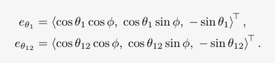

Then, the position vectors, are given explicitly as follows through algebraic accumulation:

By taking the Jacobian of each position vector, we can derive the Lagrange expression, T-V in a compact matrix formulation and use it in futher control analysis; I adopt the short hand notation for the Jacobian terms as follows:

Then, the Jacobians for the baseframe are obtained by differentiating the cartesian position vectors with respect to the generalized coordinates.






Then, we can formulate the Inertia models as follows using the azimuthal and polar basis vectors by using the following identity, which couples the state dynamics to the diagonalized inertia tensors:

Notice, that since the azimuthal coordinate does not explicitly have accumulating angles, that its inertia takes the simplified form.
The Actuator Rod Inertia, is then described using the following integral; which crudely approximates the inertia of the rod while neglecting the grooves from the actuator screw:


Then, using Autodesk Inventor inertia tensors and the analytical solution, we forlulate the inertial values as follows in the basis form for compact notation, here the theta values are added since the dynamic model is a serial manipulator.


Now, the Kinetic Energy is derived formerly using the following expression

Next, the Potential Energy is merely just the contribution of graviational potential energy, and the contributions from the DC-Actuation using the identity provided through Manhães and his affiliates. ²

As reflected by the adjusted lower index in the gravitational potential-energy summation, the base-frame contribution is omitted because its center of mass is fixed relative to the inertial reference frame. In the adopted coordinate system, the base-frame mount lies at the reference elevation, consistent with both the symbolic model and the Autodesk Inventor mass-property data. Its gravitational potential energy is therefore constant—and, with the chosen zero-potential datum, equal to zero—so it produces no generalized gravitational force when differentiated with respect to the active coordinates. Next, we need to consider the dissipation caused by the Armature resistance by considering the Rayleigh Dissipation function as follows:

Finally, because the M.M.V.1 employs KHK SH2-series geared transmissions, each angular joint is subject to a kinematic gear constraint of the following form. This relation maps the motor-side angles measured by the AS5048A magnetic encoders to the corresponding rigid-body joint angles through the prescribed gear ratio.

Then, the Augmented Lagrangian takes the following form:

The equations of motion are then explicitly derived using the traditional identity of Euler-Lagrange:

To clean up the equations of motion, the explicit version is then used to derive the canoncial form which makes the Teensy 4.1. happy considering that it now is in compact matrix form. I also use the nullspace of the constraint equations, and I have also expressed the constraint matrices A and S to further clean up the equations of motion. With the independent coordinates being defined as:

The full coordinates used in the derivation consist of:

Then, the Manipulator equation is compactly written as follows, with the


Since the system is first order in current, it can easily be decoupled as follows:

Then, since the result of the Potential Gradient contains current, it is then substituted into the dynamics as follows:

After substition, the potential gradient becomes:

Note that the coordinates here used in the current is specified as follows,

To reduce the dimensions, the equations are then written in compact matrix form, and then the nullspace is derived from this expression, resulting in a 4x1 manipulator equation.

From this expression, we derive the nullspace:
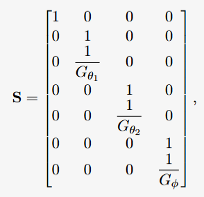
Note that this nullspace is useful since it will directly provide the full set of coordinates:
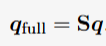
Finally, the Manipulator equation in compact form can be acknolwedged by:

With the reduced terms given as follows,

Following null-space reduction, the Euler–Lagrange equations of motion are expressed compactly as a 4x1 vector system in ℝ⁴, with one equation corresponding to each independent generalized coordinate of the M.M.V.1. For low-level implementation on the Teensy 4.1, the actuator relations are subsequently rewritten in a compact canonical duty-cycle form.

Substituting the Euler-Lagrange solutions into the Duty Cycle, we obtain the compact expression where H and K are matrices of rank 4.

Thus, the Canonical Duty Cycle is given as follows:

Control Policy
Using the canonical duty-cycle equations together with proportional–derivative feedback, a nominal low-level control policy can be constructed directly from the Euler–Lagrange model:

The system gains for this manipulator, which are BOTH used in the Teensy 4.1., and the simulations here are given as:

The controller gains listed below are used in both the Teensy 4.1 implementation and the MATLAB simulations. The radial coordinate remains under development because its sensing, calibration, and closed-loop behavior have not yet been fully validated. In contrast, the angular coordinates have demonstrated reliable experimental performance on the M.M.V.1. This is particularly true for the azimuthal coordinate, ϕ(t).
Numerical Results
The numerical results presented in this section evaluate the actuator demands predicted by the Euler--Lagrange and GDTH--PMP formulations under both static and dynamic operating conditions. The analysis includes static payload-loading surfaces, model-based holding-duty predictions, GDTH--PMP trajectory results, and an experimentally validated numerical integration of the manipulator dynamics using ode45.
Duty Cycle Validation
The static loading analysis evaluates the duty-cycle requirements of the manipulator over a range of joint configurations and payload masses. Surface plots are generated by varying the generalized coordinates while maintaining quasi static conditions. The resulting duty-cycle maps illustrate how gravitational loading, manipulator configuration, and payload mass influence the steady actuator effort required to maintain a prescribed pose. Animated surface plots further demonstrate the variation in the predicted holding duty cycles as the payload mass is increased.
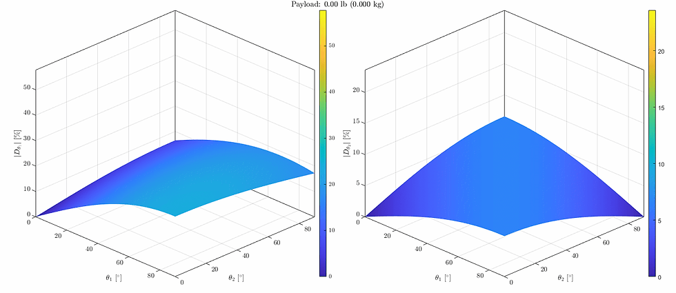
A similar trend was observed for trajectories generated using the GDTH–PMP framework, which is discussed later in this paper. The resulting state trajectories produced feasible actuator duty-cycle demands across the manipulator. For the trajectory considered here, the shoulder joint required a peak duty cycle of approximately 30% while the prismatic actuator approached 100%. The latter result is expected because the actuator nears its no-load speed along this trajectory, causing the commanded duty cycle to approach full input voltage.
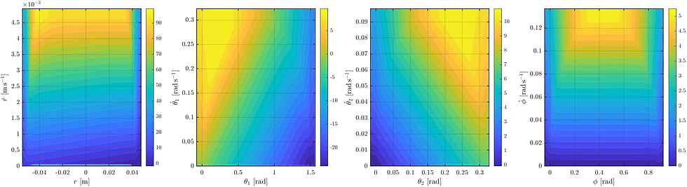
The kinematics which support this plotting behavior is shown below as follows:


Inverse Kinematics based Trajectories
The same inverse-dynamics framework may be applied when the manipulator is subjected to an arbitrary task-space path. In the present analysis, each Cartesian trajectory was converted into a generalized-coordinate trajectory using inverse-kinematics solutions computed numerically in MATLAB. The resulting histories of q, dq/dt, d2q/dt2, were then supplied directly to the electromechanical inverse-dynamics model to determine the nominal duty-cycle commands required along the path.
Ten trajectories were evaluated, each having a duration of 25 s and containing 500 samples. Across all trajectories, the numerical inverse-kinematics procedure produced a mean maximum residual norm of 5.827×10^{−10} and a mean maximum Cartesian-position error of 1.784×10^{−5 }m. The corresponding velocity solutions produced a mean maximum residual norm of 8.226×10{−20} and a mean maximum Cartesian-velocity error of 1.119× 10^{-10} m/s. These values indicate that the numerical inverse-kinematics and velocity-mapping procedures remained highly accurate across the evaluated paths.

Across nearly all evaluated trajectories, the radial linear actuator reached the imposed duty-cycle limits of

corresponding to +100% or −100% duty cycle. This result is unsurprising and should not be interpreted as a numerical anomaly. The selected UYGALAXY actuator is a 12-V, 100-mm-stroke device rated for a travel speed of only 0.2 in/s, or approximately 5 mm/s, with a nominal force rating of 188 N.³ Consequently, even moderate reference velocities demand operation near the actuator’s maximum available speed, causing the inverse electromechanical mapping to drive the normalized duty command immediately toward +1 during extension and −1 during retraction.
The radial actuator therefore constitutes the principal kinematic bottleneck of the M.M.V.1. Its sustained saturation is further influenced by the fact that the rack-and-pinion claw assembly was included as part of the gripper rigid-body model and therefore contributed directly to the gripper mass, center of mass, and inertia tensor used by the Euler–Lagrange formulation. Although the actuator operates with comparatively low measured current under the tested loading conditions, its very low no-load translational speed dominates the commanded response. Put bluntly: a 5 mm/s actuator asked to follow a faster generalized trajectory has nowhere else to go—the duty cycle must saturate.
By comparison, the revolute coordinates are driven by DOCYKE DC550 planetary gearmotors. The selected listing identifies the motor as an 18-V, 46-rpm planetary gearmotor with a nominal 550 kg cm torque designation and metal planetary transmission.⁴ These substantially faster rotary actuators can reproduce the smooth inverse-dynamics duty profiles without remaining continuously saturated.
Despite the radial saturation, the computed results remain physically meaningful. They correctly identify that the linear actuator, rather than the high-torque rotary motors, limits the speed at which the complete manipulator can execute an arbitrary coordinated path.
ODE-45 Numerical Results
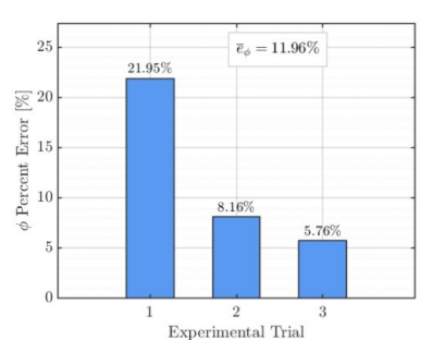
An experimental validation was conducted following completion of the colored prototype. During the test, only the azimuthal coordinate was actuated, using a commanded duty cycle of 12%, while the duty cycles applied to the remaining coordinates were set to zero. The initial conditions were obtained directly from the physical manipulator using a digital level to estimate the angular coordinates and a ruler to measure the translational position of the prismatic actuator.

The measured initial state was then supplied to the nonlinear Euler–Lagrange model and numerically integrated using MATLAB’s ode15s solver. The resulting azimuthal response was compared with the experimentally measured motion over three trials. The model produced a mean error of approximately 11%, indicating reasonable agreement between the simulated and experimental responses.
Several drivetrain effects were omitted from the numerical model, including Coulomb friction, gear backlash, gear compliance, and gravitational sag. Here, gravitational sag refers specifically to the passive downward motion observed at certain arm configurations when the electromechanical DC actuators are not energized and therefore provide no active holding torque. This behavior was not included in the model because the available motor documentation does not specify unpowered holding torque, backdrivability, or sagging characteristics. In addition, the Rayleigh dissipation function accounted only for armature-related electrical losses and did not include mechanical viscous damping. The link masses, centers of mass, and inertia tensors were obtained directly from Autodesk Inventor. Because only the azimuthal actuator was commanded during the experiment, the gradual motion observed in the remaining angular coordinates was attributed primarily to mechanical coupling within the drivetrain. This behavior was especially pronounced in the colored prototype, whose azimuthal transmission exhibited greater backlash than the final manipulator assembly. Despite these unmodeled effects, the simulated response remained reasonably
consistent with the measured experimental behavior.

Conclusion/ Future Work
In conclusion, the M.M.V.1 dynamical model produces responses that remain broadly consistent with experimental observations and provides a useful reference model for computing nominal actuator duty cycles. The formulation treats the manipulator as an approximately conservative mechanical system, with dissipation arising primarily from armature resistance within the electromechanical actuator model. Virtual springs and artificial damping terms were intentionally removed so that the controller would rely directly on the derived manipulator dynamics rather than on auxiliary restoring forces introduced to suppress or approximate dependent electromechanical states. Consequently, the resulting duty-cycle commands are obtained from the modeled inertial, Coriolis, gravitational, and back-electromotive-force contributions of the physical system itself. For the arbitrary inverse-kinematics trajectories considered, the radial actuator reached approximately 100% duty cycle during nearly every extension or retraction phase. This saturation is an expected physical result because the selected linear actuator has a listed no-load speed of only 5 mm/s. Therefore, nearly any coordinated trajectory requiring appreciable radial motion drives the actuator toward
By comparison, the rotary joints are driven by higher-speed planetary gearmotors and generally remain below sustained saturation. In future work, an LQR controller may be incorporated alongside the existing Euler–Lagrange and PD framework to improve regulation about selected equilibrium configurations. In this operating regime, Coriolis and centrifugal effects become negligible, and the holding duty cycle is governed primarily by the potential-gradient contribution required to counteract gravity.
Implementing the rigid-body model directly on the Teensy 4.1 also simplifies the separation between high-level planning and low-level control. External SLAM, vision, or task-planning systems need only transmit feasible Cartesian or joint-space references through serial communication, while the Teensy evaluates the corresponding inverse-dynamics and feedback commands in real time. A reduced high-level representation may therefore describe the desired end-effector motion using only Cartesian coordinates, such as x, y, and z, provided that inverse kinematics is used to recover a feasible joint-space trajectory. Once a kinematically valid and dynamically reasonable path is supplied, the Euler–Lagrange feedforward model performs most of the nominal control effort, while the feedback controller compensates for modeling errors, disturbances, and imperfect tracking.
The MATLAB code for these simulations, can be provided below as follows:
1.)N. S. Nise, Control Systems Engineering, 7th ed. Hoboken, NJ, USA: John Wiley & Sons, 2015, p. 80.
2.) W. Manhães, R. Sampaio, R. Lima, P. Hagedorn, and J.-F. Deü, “Lagrangians for electromechanical systems,” Mecánica Computacional, vol. 36, no. 42, pp. 1911–1934, 2018. [Online]. Available: https://hal.science/hal-04102439v1/document
3.) UYGALAXY, “12 V mini electric linear actuator, 4-in stroke, 188 N/42 lb, speed 0.2 in/s, waterproof metal motion actuator,” Amazon.com. [Online]. Available: https://www.amazon.com/UYGALAXY-Electric-Actuator-Waterproof-Mounting/dp/B0BPC79768
4.) DOCYKE, “DC planet gear motor (550KG.CM), 6V/12V/18V/22V, 200 W high-torque mini metal reduction geared motor for DIY robot,” Amazon.com. [Online]. Available: https://www.amazon.com/550KG-CM-6v12V18V24v-Reduction-Rotating-Curtain/dp/B0DZ246RQ5